
In order to explain how we calculate expected retention and expected customer lifetime value (eCLV) for subscriptions we will take a tour through our imaginary shop named Charlie’s chocolate store. Charlie is selling chocolate box subscriptions on his Shopify website and is very determined to be the best business owner in chocolate history. This is why he wants to carefully measure all of the most important metrics, including the expected customer lifetime value.
A chocolate box in Charlie’s store costs $20. You can only buy it on a monthly subscription, meaning you are automatically charged for one box each month until you cancel. You can cancel your subscription any point of time and from that moment on no future charges for your subscription will be processed.
Charlie started selling subscriptions in January 2020. A total of 1000 customers bought a subscription in the initial month generating $20 000 of revenue and Charlie started analysing this cohort (group) of users through time. In February 373 cancelled, leaving 627 to order again. In March 156 additional customers cancelled, leaving only 471 to order again and so on.
After five months, Charlie looks at the data in the table and plot below. He wants to know what his expected CLV would be for this cohort.
| Month 0 | Month 1 | Month 2 | Month 3 | Month 4 | Month 5 |
| 1000 | 627 | 471 | 385 | 328 | ??? |
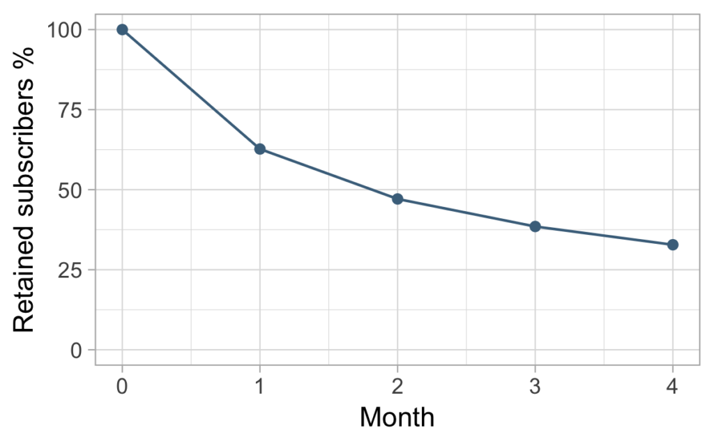
Since he knows they are paying $20 per order, the only thing he really needs to estimate is how many of them will keep ordering in the following months. He draws a line showing the percentage of users remaining each month and asks himself: “How will this line continue to decline?” Or put even more simply: “How long in average do users stay?.
So instead of looking for ways to estimate expected lifetime value (eCLV), we can solve the equivalent problem of expected retention (eRet) using the connection
eCLV = (eRet +1) * $20.
Note that in more general terms, the formula would look more like
eCLV = (eRet / period + 1) * AOV,
where period is the subscription period in months and AOV the average order value. The same principle can also be applied for daily and weekly periods. For demonstration purposes we will stick to our simple case with monthly periods.
Helping Charlie to draw the line
First option that comes to a mathematician’s mind in problems like this is probably curve fitting. So what kind of function would be suitable to use here? Obviously not a straight line, but maybe something like an exponential function would work. Instead of trying random functions without really knowing what we are doing, we can derive the formula using a probabilistic approach. We will start with a simple model of constant churn.
A constant churn estimation
Let’s assume that each month each customer has the same probability p to churn. In this case the probability for churning in the first month would be p, in the second month (1-p)p,in the third month (1-p)^2*p and so on. This means that, out of 1000 customers which started in January, we would expect 1000*p to churn in February, 1000*(1-p)*p to churn in March, 1000*(1-p)^2*p to churn in April and so on. Taking a look at the data in the table below, we ask ourselves how to calculate the churn rate p that matches the data we have so far the best.
Months since start | Churned Customers | Estimated churned customers |
| 1 | 373 | 1000*p |
| 2 | 156 | 1000*(1-p)*p |
| 3 | 86 | 1000*(1-p)^2*p |
| 4 | 57 | 1000*(1-p)^3*p |
| >=5 | 328 | 1000*(1-p)^4 |
The method for choosing p is not unified, but the one mostly used is the MLE method (maximum likelihood estimator) which is commonly used in multiple statistical problems. An alternative approach could be using the least squares estimator, i.e. minimizing the sum of the squares of the residuals. We will not go into detail about these methods here since they are widely used in statistics and covered with exhausting materials on the internet.
If you would estimate p in this case, using the MLE method, you would get p_MLE = 27.1%. It’s interesting to see how the estimated churned customers for p = 27.1% look like, so let’s update our table:
Months since start |
Churned customers |
Estimated ch. cust. p = 27.1% |
| 1 | 373 | 271 |
| 2 | 156 | 198 |
| 3 | 86 | 144 |
| 4 | 57 | 105 |
| >=5 | 328 | 282 |
This table tells us the following: if the churn rate in reality was constant and equal to 27.1%, our data would be approximately equal to the third column.
Let’s also take a look at the predicted curve compared to the real data.
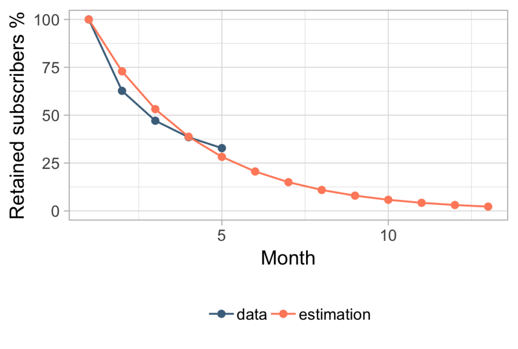
Looking at the plot without the future data, it’s hard to tell if this estimation is a good approach for solving our problem. But before we go into evaluating the model, let’s see how we would use it to calculate the estimated retention. First we remind ourselves that, given the churn is constant for each month, we know that the probability of churning in month m is equal to:
P(customer retained exactly m months) = P(customer churns in month m) = (1-p)^(m-1)*p. So the average subscription period of a customer would be calculated in the following way: eRet = 1*P(Ret = 1) + 2*P(Ret = 2) + 3*P(Ret = 3) + …. = 1*p + 2*(1-p)*p + 3*(1-p)^2*p + … = . . . = 1/p (We again skipped the calculations here, but if you are familiar with indefinite sums you will easily see the derivation of the geometric series here which leads you to solving this sum.
This approach is what we mostly saw being used in practice and most commonly seen in other blog posts. Even if the mathematics behind it is moderately complicated, the final formula is really simple to remember: retention = 1 / churn. All in all, this seemed like a really nice and practical solution and Charlie loved it. But after a year passed he wanted to check how his prediction compared to actual measured data and he got this picture below.
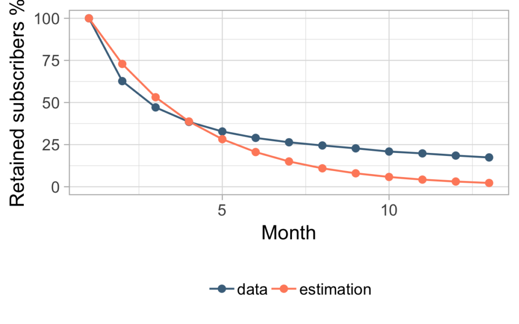
First, Charlie was happy because in the future he obviously earned more than he expected. But afterwards he started wondering why his prediction was so wrong. He noticed that the model had lower churn rates in the first couple of months compared to the real data, while in the future the churn rate used in the model was obviously much higher than the ones measured in our data.Ultimately, assuming that the churn rate is constant over time was not really fitting the real picture.
A churn rate that varies
How can we introduce variability in the concept of churn rate and improve our model? Fader and Hardie (Fader, Peter S. and Bruce G.S.Hardie (2007), “How to Project Customer Retention”, Journal of Interactive Marketing) developed what they called a beta-geometric model. The beta-geometric model is based on the basic geometric model explained above expanded by allowing additional flexibility in p: the churn rate p is not considered a constant between 0 and 1 anymore, but a random variable with values between 0 and 1.
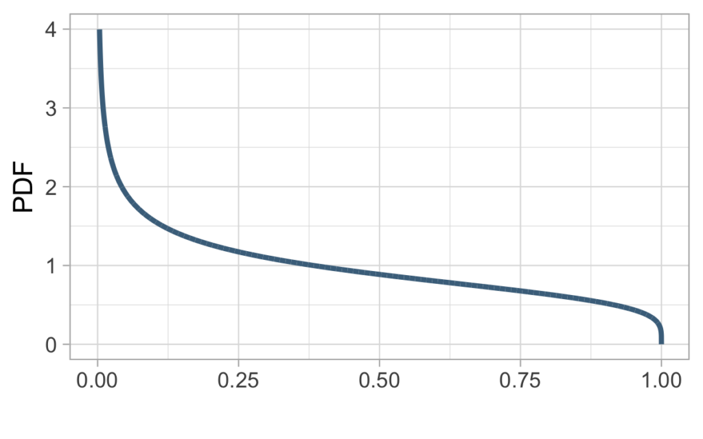
For example the initial distribution of p can look like one of the examples on the picture below.
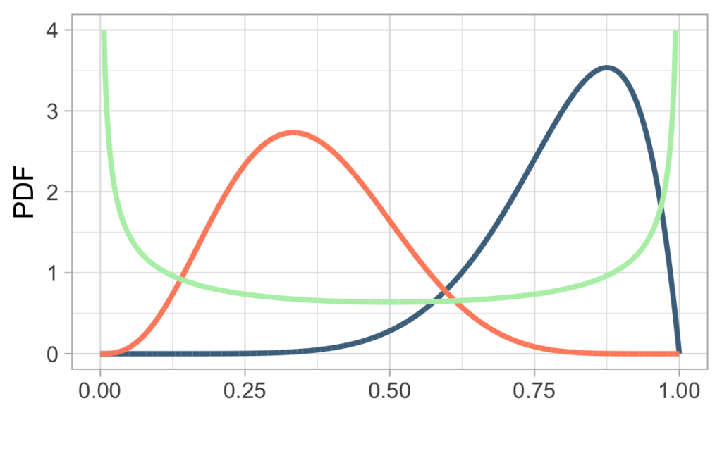
The orange distribution would mean that most of the customers have a moderate churn rate somewhere between 0.2 and 0.6, but there is also a small part of customers with very high or very low churn rates. On the other hand, the green distribution shows an example with a lot of extreme customers, in sense that they have very high or very low churn rates. The blue line is a case of very high churn rates, a huge proportion of customers have a churn probability higher than 0.5.
But why should churn rates vary among customers? Fader and Hardie explain this through people having different tastes and characters which makes them more or less likely to like the product and thus churn. So the variability of p is a consequence of having a lot of different customers subscribe to a product to try it out, not knowing if this product will suit their needs. How customers react to the product determines the shape of the distribution.
If the product is really bad, then the churn rates might be similar to the blue distribution, i.e. most of them will churn really soon since they have a high churn probability. On the other hand, if your product is good, maybe we would expect something like the orange distribution. A green distribution could be something like a love-it-or-hate-it product.
In any case, as time passes, most of the customers with high churn probability will churn and only loyal customers with low churn rates will remain, which leads to a decline in overall churn rate. Let’s go through example below to explain this in more detail.
Old people don’t like chocolate
We were saying that people have different churn rates because there are different types of people. Let’s look at an oversimplified example from our imaginary world where there are only two kinds of people, old and young people, and old people like chocolate less than young people. This is why old people are more likely to churn from Charlie’s subscriptions. In our imaginary world we know that young people have exactly p_young = 0.2 and old people have p_old = 0.4. Additionally, from 1000 customers Charlie started with, exactly 500 are old and 500 are young, so the average churn rate at the beginning is p = 0.3.
Let’s take a look how many of them would remain over time:
| Month 1 | Month 2 | Month 3 | Month 4 | Month 5 | |
| Old | 500 | 300 | 120 | 48 | 19 |
| Young | 500 | 400 | 320 | 256 | 205 |
| Avg churn rate: | 30% | 29% | 25% | 23% | 22% |
Interestingly, you can see that the average churn rate decreases over time! Like we mentioned before, this is the side effect of having different customers: most young people stay and more and more old people leave. This is why in reality we often see average churn rates stabilizing over time.
Estimating the distribution of p
So far we explained why we want to model p with a distribution on [0,1], but we didn’t yet say how exactly this can be achieved. Since we have no idea how the initial distribution looks like in the beginning, we want a flexible model which will allow all kinds of shapes to be taken into account. This is where the beta distribution comes in. Beta distributions can handle a lot of different shapes on [0,1] and are therefore suitable for problems like this. The blue, green and orange examples above are only a couple of examples of beta distributions.
This is why Fader and Hardie chose to model the churn rate as:
p ~beta(a, b),
where a and b are the shape parameters. In the same manner as we were estimating p in the simple geometric example, we now have to estimate the parameters a and b which determine the shape for the distribution of p.
Previously we chose p which suits the data in the table below the most (the MLE predictor):
Months since start | Churned Customers | Estimated churned customers |
| 1 | 373 | 1000*p |
| 2 | 156 | 1000*(1-p)*p |
| 3 | 86 | 1000*(1-p)**2**p |
| 4 | 57 | 1000*(1-p)**3**p |
| >=5 | 328 | 1000*(1-p)**4 |
Now we have a similar situation, only instead of p we have some more complicated terms depending on a, b.
Like previously, we can use the MLE method to estimate a and b, but because of the complexity of the calculations we won’t present the formulas here. In case you are interested in specifics, you can take a look at Fader and Hardies work where all the calculations are precisely explained.
Applied to our data we get a_MLE = 0.73 and b_MLE = 1.23 and the corresponding beta distribution shown on the picture below.
According to the distribution which is more heavily concentrated on the left side, we expect that among the 1000 initial customers more of them had low churn probability.
Let’s now look at the data vs estimation graph. If Charlie would have used this method after five months of data he would have gotten the following estimation:
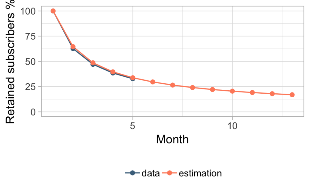
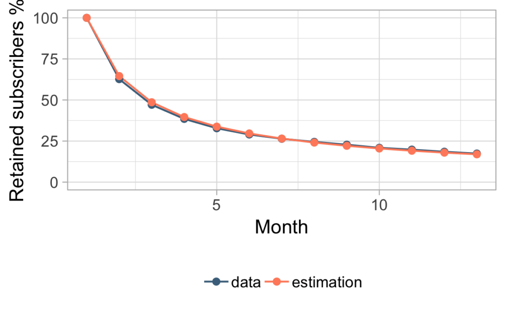
Since we have two estimated parameters here, it’s not unreasonable to get such a good fit for the data. Of course, the real question is, how does this estimation compare to future data? Looking at the comparison below, you can see that Charlie can now be completely satisfied.
Is this as complicated as it gets?
The model shown above is a great starting point, but when you get to real use cases there are lots of additional things you need to take care of – multiple subscription periods, different AOVs, multiple items, different payment options and so on. Moving on, we get to purchases on a one-time basis where the definition of churn is not clear, the period between purchases is not fixed, and things get even more complicated. Luckily, with RAPP we’ve got you covered.


No comment yet, add your voice below!